DataFrame(数据帧)
DataFrame是带有标签的二维数据结构,列的类型可能不同。你可以把它想象成一个电子表格或SQL表,或者 Series 对象的字典。它一般是最常用的pandas对象。像 Series 一样,DataFrame 接受许多不同类型的输入:
- 一维数组,列表,字典或 Series 的字典
- 二维 numpy.ndarray
- 结构化或记录 ndarray
Series- 另一个
DataFrame
和数据一起,您可以选择传递index(行标签)和columns(列标签)参数。如果传递索引或列,则会用于生成的DataFrame的索引或列。因此,Series 的字典加上特定索引将丢弃所有不匹配传入索引的数据。
如果轴标签未通过,则它们将基于常识规则从输入数据构造。
来自 Series 或字典的字典
结果的index是各种系列索引的并集。如果有任何嵌套的词典,这些将首先转换为Series。如果列没有传递,这些列将是字典的键的有序列表。
In [32]: d = {'one' : pd.Series([1., 2., 3.], index=['a', 'b', 'c']),
   ....:      'two' : pd.Series([1., 2., 3., 4.], index=['a', 'b', 'c', 'd'])}
   ....:

In [33]: df = pd.DataFrame(d)

In [34]: df
Out[34]:
   one  two
a  1.0  1.0
b  2.0  2.0
c  3.0  3.0
d  NaN  4.0

In [35]: pd.DataFrame(d, index=['d', 'b', 'a'])
Out[35]:
   one  two
d  NaN  4.0
b  2.0  2.0
a  1.0  1.0

In [36]: pd.DataFrame(d, index=['d', 'b', 'a'], columns=['two', 'three'])
Out[36]:
   two three
d  4.0   NaN
b  2.0   NaN
a  1.0   NaN
通过访问index和column属性可以分别访问行和列标签:
注意
同时传入一组特定的列和数据的字典时,传入的列将覆盖字典中的键。
In [37]: df.index
Out[37]: Index([u'a', u'b', u'c', u'd'], dtype='object')

In [38]: df.columns
Out[38]: Index([u'one', u'two'], dtype='object')
来自 ndarrays / lists 的字典
ndarrays 必须长度相同。如果传入了索引,它必须也与数组长度相同。如果没有传入索引,结果将是range(n),其中n是数组长度。
In [39]: d = {'one' : [1., 2., 3., 4.],
   ....:      'two' : [4., 3., 2., 1.]}
   ....:

In [40]: pd.DataFrame(d)
Out[40]:
   one  two
0  1.0  4.0
1  2.0  3.0
2  3.0  2.0
3  4.0  1.0

In [41]: pd.DataFrame(d, index=['a', 'b', 'c', 'd'])
Out[41]:
   one  two
a  1.0  4.0
b  2.0  3.0
c  3.0  2.0
d  4.0  1.0
来自结构化或记录数组
这种情况与数组的字典相同。
In [42]: data = np.zeros((2,), dtype=[('A', 'i4'),('B', 'f4'),('C', 'a10')])

In [43]: data[:] = [(1,2.,'Hello'), (2,3.,"World")]

In [44]: pd.DataFrame(data)
Out[44]:
   A    B      C
0  1  2.0  Hello
1  2  3.0  World

In [45]: pd.DataFrame(data, index=['first', 'second'])
Out[45]:
        A    B      C
first   1  2.0  Hello
second  2  3.0  World

In [46]: pd.DataFrame(data, columns=['C', 'A', 'B'])
Out[46]:
       C  A    B
0  Hello  1  2.0
1  World  2  3.0
注意
DataFrame并不打算完全类似二维NumPy ndarray一样。
来自字典的数组
In [47]: data2 = [{'a': 1, 'b': 2}, {'a': 5, 'b': 10, 'c': 20}]

In [48]: pd.DataFrame(data2)
Out[48]:
   a   b     c
0  1   2   NaN
1  5  10  20.0

In [49]: pd.DataFrame(data2, index=['first', 'second'])
Out[49]:
        a   b     c
first   1   2   NaN
second  5  10  20.0

In [50]: pd.DataFrame(data2, columns=['a', 'b'])
Out[50]:
   a   b
0  1   2
1  5  10
来自元组的字典
您可以通过传递元组字典来自动创建多索引的 DataFrame
In [51]: pd.DataFrame({('a', 'b'): {('A', 'B'): 1, ('A', 'C'): 2},
   ....:               ('a', 'a'): {('A', 'C'): 3, ('A', 'B'): 4},
   ....:               ('a', 'c'): {('A', 'B'): 5, ('A', 'C'): 6},
   ....:               ('b', 'a'): {('A', 'C'): 7, ('A', 'B'): 8},
   ....:               ('b', 'b'): {('A', 'D'): 9, ('A', 'B'): 10}})
   ....:
Out[51]:
       a              b
       a    b    c    a     b
A B  4.0  1.0  5.0  8.0  10.0
  C  3.0  2.0  6.0  7.0   NaN
  D  NaN  NaN  NaN  NaN   9.0
来自单个 Series
结果是一个 DataFrame,索引与输入的 Series 相同,并且单个列的名称是 Series 的原始名称(仅当没有提供其他列名时)。
缺失数据
在缺失数据部分中,将对此主题进行更多说明。为了构造具有缺失数据的DataFrame,请将np.nan用于缺失值。或者,您可以将numpy.MaskedArray作为数据参数传递给DataFrame构造函数,它屏蔽的条目将视为缺失值。
备选构造函数
DataFrame.from_dict
DataFrame.from_dict接受字典的字典或类似数组的序列的字典,并返回DataFrame。它的操作类似DataFrame的构造函数,除了默认情况下为'columns'的orient参数,但它可以设置为'index',以便将字典的键用作行标签。
DataFrame.from_records
DataFrame.from_records首届元组的列表或带有结构化dtype的ndarray。它的工作方式类似于正常DataFrame构造函数,除了索引可能是结构化dtype的特定字段。例如:
In [52]: data
Out[52]:
array([(1, 2.0, 'Hello'), (2, 3.0, 'World')],
      dtype=[('A', '<i4'), ('B', '<f4'), ('C', 'S10')])

In [53]: pd.DataFrame.from_records(data, index='C')
Out[53]:
       A    B
C
Hello  1  2.0
World  2  3.0
DataFrame.from_items
DataFrame.from_items类似于字典的构造函数,它接受键 值对的序列,其中的键是列标签(或在orient ='index'的情况下是行标签),值是列的值(或行的值)。对于构建列为特定的顺序的DataFrame,而不必传递明确的列的列表,它非常有用:
In [54]: pd.DataFrame.from_items([('A', [1, 2, 3]), ('B', [4, 5, 6])])
Out[54]:
   A  B
0  1  4
1  2  5
2  3  6
如果您传入orient='index',键将是行标签。但在这种情况下,您还必须传递所需的列名称:
In [55]: pd.DataFrame.from_items([('A', [1, 2, 3]), ('B', [4, 5, 6])],
   ....:                         orient='index', columns=['one', 'two', 'three'])
   ....:
Out[55]:
   one  two  three
A    1    2      3
B    4    5      6
列的选取、添加、删除
你可以在语义上,将 DataFrame 当做 Series 对象的字典来处理。列的获取,设置和删除的方式与字典操作的语法相同:
In [56]: df['one']
Out[56]:
a    1.0
b    2.0
c    3.0
d    NaN
Name: one, dtype: float64

In [57]: df['three'] = df['one'] * df['two']

In [58]: df['flag'] = df['one'] > 2

In [59]: df
Out[59]:
   one  two  three   flag
a  1.0  1.0    1.0  False
b  2.0  2.0    4.0  False
c  3.0  3.0    9.0   True
d  NaN  4.0    NaN  False
列可以像字典一样删除或弹出:
In [60]: del df['two']

In [61]: three = df.pop('three')

In [62]: df
Out[62]:
   one   flag
a  1.0  False
b  2.0  False
c  3.0   True
d  NaN  False
当插入一个标量值时,它自然会广播来填充该列:
In [63]: df['foo'] = 'bar'

In [64]: df
Out[64]:
   one   flag  foo
a  1.0  False  bar
b  2.0  False  bar
c  3.0   True  bar
d  NaN  False  bar
当插入的 Series 与 DataFrame 的索引不同时,它将适配 DataFrame 的索引:
In [65]: df['one_trunc'] = df['one'][:2]

In [66]: df
Out[66]:
   one   flag  foo  one_trunc
a  1.0  False  bar        1.0
b  2.0  False  bar        2.0
c  3.0   True  bar        NaN
d  NaN  False  bar        NaN
您可以插入原始的ndarray,但它们的长度必须匹配DataFrame的索引的长度。
默认情况下,列在末尾插入。insert函数可用于在列中的特定位置插入:
In [67]: df.insert(1, 'bar', df['one'])

In [68]: df
Out[68]:
   one  bar   flag  foo  one_trunc
a  1.0  1.0  False  bar        1.0
b  2.0  2.0  False  bar        2.0
c  3.0  3.0   True  bar        NaN
d  NaN  NaN  False  bar        NaN
使用方法链来创建新的列
版本0.16.0中的新功能。
受dplyr的mutate动词的启发,DataFrame 拥有assign()方法,允许您轻易创建新的列,它可能从现有列派生。
In [69]: iris = pd.read_csv('data/iris.data')

In [70]: iris.head()
Out[70]:
   SepalLength  SepalWidth  PetalLength  PetalWidth         Name
0          5.1         3.5          1.4         0.2  Iris-setosa
1          4.9         3.0          1.4         0.2  Iris-setosa
2          4.7         3.2          1.3         0.2  Iris-setosa
3          4.6         3.1          1.5         0.2  Iris-setosa
4          5.0         3.6          1.4         0.2  Iris-setosa

In [71]: (iris.assign(sepal_ratio = iris['SepalWidth'] / iris['SepalLength'])
   ....:      .head())
   ....:
Out[71]:
   SepalLength  SepalWidth  PetalLength  PetalWidth         Name  sepal_ratio
0          5.1         3.5          1.4         0.2  Iris-setosa       0.6863
1          4.9         3.0          1.4         0.2  Iris-setosa       0.6122
2          4.7         3.2          1.3         0.2  Iris-setosa       0.6809
3          4.6         3.1          1.5         0.2  Iris-setosa       0.6739
4          5.0         3.6          1.4         0.2  Iris-setosa       0.7200
上面是插入预计算值的示例。我们还可以传递函数作为参数,这个函数会在 DataFrame 上调用,结果会添加给 DataFrame。
In [72]: iris.assign(sepal_ratio = lambda x: (x['SepalWidth'] /
   ....:                                      x['SepalLength'])).head()
   ....:
Out[72]:
   SepalLength  SepalWidth  PetalLength  PetalWidth         Name  sepal_ratio
0          5.1         3.5          1.4         0.2  Iris-setosa       0.6863
1          4.9         3.0          1.4         0.2  Iris-setosa       0.6122
2          4.7         3.2          1.3         0.2  Iris-setosa       0.6809
3          4.6         3.1          1.5         0.2  Iris-setosa       0.6739
4          5.0         3.6          1.4         0.2  Iris-setosa       0.7200
assign 始终返回数据的副本,而保留原始DataFrame不变。
传递可调用对象,而不是要插入的实际值,当您没有现有 DataFrame 的引用时,它很有用。在操作链中使用assign时,这很常见。
In [73]: (iris.query('SepalLength > 5')
   ....:      .assign(SepalRatio = lambda x: x.SepalWidth / x.SepalLength,
   ....:              PetalRatio = lambda x: x.PetalWidth / x.PetalLength)
   ....:      .plot(kind='scatter', x='SepalRatio', y='PetalRatio'))
   ....:
Out[73]: <matplotlib.axes._subplots.AxesSubplot at 0x7ff286891b50>
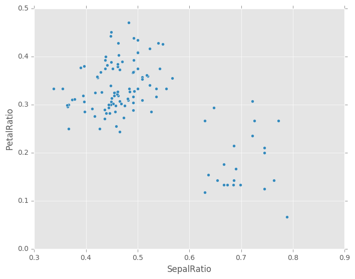
由于传入了一个函数,因此该函数在 DataFrame 上求值。重要的是,这个 DataFrame 已经过滤为 sepal 长度大于 5 的那些行。首先进行过滤,然后计算比值。这是一个示例,其中我们没有被过滤的 DataFrame的可用引用。
assign函数的参数是**kwargs。键是新字段的列名称,值是要插入的值(例如,Series或NumPy数组),或者是个函数,它在DataFrame上调用。返回原始DataFrame的副本,它插入了新值。
警告
由于assign的函数签名为**kwargs,因此不能保证在产生的DataFrame中,新列的顺序与传递的顺序一致。为了使事情可预测,条目按字典序(按键)插入到 DataFrame 的末尾。
首先计算所有表达式,然后赋值。因此,在assign的同一调用中,您不能引用要赋值的另一列。例如:
In [74]: # Don't do this, bad reference to `C`
        df.assign(C = lambda x: x['A'] + x['B'],
                  D = lambda x: x['A'] + x['C'])
In [2]: # Instead, break it into two assigns
        (df.assign(C = lambda x: x['A'] + x['B'])
           .assign(D = lambda x: x['A'] + x['C']))
索引 / 选取
索引的基本方式如下:
| 操作 | 语法 | 结果 |
|---|---|---|
| 选择列 | df[col] |
Series |
| 按标签选择行 | df.loc[label] |
Series |
| 按整数位置选择行 | df.iloc[loc] |
Series |
| 对行切片 | df[5:10] |
DataFrame |
| 通过布尔向量选择行 | df[bool_vec] |
DataFrame |
例如,行的选择返回 Series,其索引是 DataFrame 的列:
In [75]: df.loc['b']
Out[75]:
one              2
bar              2
flag         False
foo            bar
one_trunc        2
Name: b, dtype: object

In [76]: df.iloc[2]
Out[76]:
one             3
bar             3
flag         True
foo           bar
one_trunc     NaN
Name: c, dtype: object
对于更复杂的基于标签的索引和切片的更详尽的处理,请参阅索引章节。我们将在重索引章节中,强调重索引/适配新标签集的基本原理。
数据对齐和算术
DataFrame对象之间的数据自动按照列和索引(行标签)对齐。同样,生成的对象具有列和行标签的并集。
In [77]: df = pd.DataFrame(np.random.randn(10, 4), columns=['A', 'B', 'C', 'D'])

In [78]: df2 = pd.DataFrame(np.random.randn(7, 3), columns=['A', 'B', 'C'])

In [79]: df + df2
Out[79]:
        A       B       C   D
0  0.5222  0.3225 -0.7566 NaN
1 -0.8441  0.2334  0.8818 NaN
2 -2.2079 -0.1572 -0.3875 NaN
3  2.8080 -1.0927  1.0432 NaN
4 -1.7511 -2.0812  2.7477 NaN
5 -3.2473 -1.0850  0.7898 NaN
6 -1.7107  0.0661  0.1294 NaN
7     NaN     NaN     NaN NaN
8     NaN     NaN     NaN NaN
9     NaN     NaN     NaN NaN
执行 DataFrame和Series之间的操作时,默认行为是,将Dataframe 的列索引与 Series 对齐,从而按行广播。例如:
In [80]: df - df.iloc[0]
Out[80]:
        A       B       C       D
0  0.0000  0.0000  0.0000  0.0000
1 -2.6396 -1.0702  1.7214 -0.7896
2 -2.7662 -1.6918  2.2776 -2.5401
3  0.8679 -3.5247  1.9365 -0.1331
4 -1.9883 -3.2162  2.0464 -1.0700
5 -3.3932 -4.0976  1.6366 -2.1635
6 -1.3668 -1.9572  1.6523 -0.7191
7 -0.7949 -2.1663  0.9706 -2.6297
8 -0.8383 -1.3630  1.6702 -2.0865
9  0.8588  0.0814  3.7305 -1.3737
在处理时间序列数据的特殊情况下,DataFrame索引也包含日期,广播是按列的方式:
In [81]: index = pd.date_range('1/1/2000', periods=8)

In [82]: df = pd.DataFrame(np.random.randn(8, 3), index=index, columns=list('ABC'))

In [83]: df
Out[83]:
                 A       B       C
2000-01-01  0.2731  0.3604 -1.1515
2000-01-02  1.1577  1.4787 -0.6528
2000-01-03 -0.7712  0.2203 -0.5739
2000-01-04 -0.6356 -1.1703 -0.0789
2000-01-05 -1.4687  0.1705 -1.8796
2000-01-06 -1.2037  0.9568 -1.1383
2000-01-07 -0.6540 -0.2169  0.3843
2000-01-08 -2.1639 -0.8145 -1.2475

In [84]: type(df['A'])
Out[84]: pandas.core.series.Series

In [85]: df - df['A']
Out[85]:
            2000-01-01 00:00:00  2000-01-02 00:00:00  2000-01-03 00:00:00  \
2000-01-01                  NaN                  NaN                  NaN
2000-01-02                  NaN                  NaN                  NaN
2000-01-03                  NaN                  NaN                  NaN
2000-01-04                  NaN                  NaN                  NaN
2000-01-05                  NaN                  NaN                  NaN
2000-01-06                  NaN                  NaN                  NaN
2000-01-07                  NaN                  NaN                  NaN
2000-01-08                  NaN                  NaN                  NaN

            2000-01-04 00:00:00 ...  2000-01-08 00:00:00   A   B   C
2000-01-01                  NaN ...                  NaN NaN NaN NaN
2000-01-02                  NaN ...                  NaN NaN NaN NaN
2000-01-03                  NaN ...                  NaN NaN NaN NaN
2000-01-04                  NaN ...                  NaN NaN NaN NaN
2000-01-05                  NaN ...                  NaN NaN NaN NaN
2000-01-06                  NaN ...                  NaN NaN NaN NaN
2000-01-07                  NaN ...                  NaN NaN NaN NaN
2000-01-08                  NaN ...                  NaN NaN NaN NaN

[8 rows x 11 columns]
警告
df - df['A']
现已弃用,将在以后的版本中删除。复现此行为的首选方法是
df.sub(df['A'], axis=0)
对于显式控制匹配和广播行为,请参阅灵活的二元运算一节。
标量的操作正如你的预期:
In [86]: df * 5 + 2
Out[86]:
                 A       B       C
2000-01-01  3.3655  3.8018 -3.7575
2000-01-02  7.7885  9.3936 -1.2641
2000-01-03 -1.8558  3.1017 -0.8696
2000-01-04 -1.1781 -3.8513  1.6056
2000-01-05 -5.3437  2.8523 -7.3982
2000-01-06 -4.0186  6.7842 -3.6915
2000-01-07 -1.2699  0.9157  3.9217
2000-01-08 -8.8194 -2.0724 -4.2375

In [87]: 1 / df
Out[87]:
                 A       B        C
2000-01-01  3.6616  2.7751  -0.8684
2000-01-02  0.8638  0.6763  -1.5318
2000-01-03 -1.2967  4.5383  -1.7424
2000-01-04 -1.5733 -0.8545 -12.6759
2000-01-05 -0.6809  5.8662  -0.5320
2000-01-06 -0.8308  1.0451  -0.8785
2000-01-07 -1.5291 -4.6113   2.6019
2000-01-08 -0.4621 -1.2278  -0.8016

In [88]: df ** 4
Out[88]:
                  A       B           C
2000-01-01   0.0056  0.0169  1.7581e+00
2000-01-02   1.7964  4.7813  1.8162e-01
2000-01-03   0.3537  0.0024  1.0849e-01
2000-01-04   0.1632  1.8755  3.8733e-05
2000-01-05   4.6534  0.0008  1.2482e+01
2000-01-06   2.0995  0.8382  1.6789e+00
2000-01-07   0.1829  0.0022  2.1819e-02
2000-01-08  21.9244  0.4401  2.4219e+00
布尔运算符也同样有效:
In [89]: df1 = pd.DataFrame({'a' : [1, 0, 1], 'b' : [0, 1, 1] }, dtype=bool)

In [90]: df2 = pd.DataFrame({'a' : [0, 1, 1], 'b' : [1, 1, 0] }, dtype=bool)

In [91]: df1 & df2
Out[91]:
       a      b
0  False  False
1  False   True
2   True  False

In [92]: df1 | df2
Out[92]:
      a     b
0  True  True
1  True  True
2  True  True

In [93]: df1 ^ df2
Out[93]:
       a      b
0   True   True
1   True  False
2  False   True

In [94]: -df1
Out[94]:
       a      b
0  False   True
1   True  False
2  False  False
转置
对于转置,访问T属性(transpose函数也是),类似于ndarray:
# only show the first 5 rows
In [95]: df[:5].T
Out[95]:
   2000-01-01  2000-01-02  2000-01-03  2000-01-04  2000-01-05
A      0.2731      1.1577     -0.7712     -0.6356     -1.4687
B      0.3604      1.4787      0.2203     -1.1703      0.1705
C     -1.1515     -0.6528     -0.5739     -0.0789     -1.8796
DataFrame 与 NumPy 函数的互操作
逐元素的 NumPy ufunc(log,exp,sqrt,...)和各种其他NumPy函数可以无缝用于DataFrame,假设其中的数据是数字:
In [96]: np.exp(df)
Out[96]:
                 A       B       C
2000-01-01  1.3140  1.4338  0.3162
2000-01-02  3.1826  4.3873  0.5206
2000-01-03  0.4625  1.2465  0.5633
2000-01-04  0.5296  0.3103  0.9241
2000-01-05  0.2302  1.1859  0.1526
2000-01-06  0.3001  2.6034  0.3204
2000-01-07  0.5200  0.8050  1.4686
2000-01-08  0.1149  0.4429  0.2872

In [97]: np.asarray(df)
Out[97]:
array([[ 0.2731,  0.3604, -1.1515],
       [ 1.1577,  1.4787, -0.6528],
       [-0.7712,  0.2203, -0.5739],
       [-0.6356, -1.1703, -0.0789],
       [-1.4687,  0.1705, -1.8796],
       [-1.2037,  0.9568, -1.1383],
       [-0.654 , -0.2169,  0.3843],
       [-2.1639, -0.8145, -1.2475]])
DataFrame上的dot方法实现了矩阵乘法:
In [98]: df.T.dot(df)
Out[98]:
         A       B       C
A  11.1298  2.8864  6.0015
B   2.8864  5.3895 -1.8913
C   6.0015 -1.8913  8.6204
类似地,Series上的dot方法实现了点积:
In [99]: s1 = pd.Series(np.arange(5,10))

In [100]: s1.dot(s1)
Out[100]: 255
DataFrame不打算作为ndarray的替代品,因为它的索引语义和矩阵是非常不同的。
控制台展示
非常大的DataFrames将被截断,来在控制台中展示。您也可以使用info()取得摘要。(这里我从plyr R软件包中,读取CSV版本的棒球数据集):
In [101]: baseball = pd.read_csv('data/baseball.csv')

In [102]: print(baseball)
       id     player  year  stint  ...   hbp   sh   sf  gidp
0   88641  womacto01  2006      2  ...   0.0  3.0  0.0   0.0
1   88643  schilcu01  2006      1  ...   0.0  0.0  0.0   0.0
..    ...        ...   ...    ...  ...   ...  ...  ...   ...
98  89533   aloumo01  2007      1  ...   2.0  0.0  3.0  13.0
99  89534  alomasa02  2007      1  ...   0.0  0.0  0.0   0.0

[100 rows x 23 columns]

In [103]: baseball.info()
<class 'pandas.core.frame.DataFrame'>
RangeIndex: 100 entries, 0 to 99
Data columns (total 23 columns):
id        100 non-null int64
player    100 non-null object
year      100 non-null int64
stint     100 non-null int64
team      100 non-null object
lg        100 non-null object
g         100 non-null int64
ab        100 non-null int64
r         100 non-null int64
h         100 non-null int64
X2b       100 non-null int64
X3b       100 non-null int64
hr        100 non-null int64
rbi       100 non-null float64
sb        100 non-null float64
cs        100 non-null float64
bb        100 non-null int64
so        100 non-null float64
ibb       100 non-null float64
hbp       100 non-null float64
sh        100 non-null float64
sf        100 non-null float64
gidp      100 non-null float64
dtypes: float64(9), int64(11), object(3)
memory usage: 18.0+ KB
但是,使用to_string将返回表格形式的DataFrame的字符串表示,但并不总是适合控制台宽度:
In [104]: print(baseball.iloc[-20:, :12].to_string())
       id     player  year  stint team  lg    g   ab   r    h  X2b  X3b
80  89474  finlest01  2007      1  COL  NL   43   94   9   17    3    0
81  89480  embreal01  2007      1  OAK  AL    4    0   0    0    0    0
82  89481  edmonji01  2007      1  SLN  NL  117  365  39   92   15    2
83  89482  easleda01  2007      1  NYN  NL   76  193  24   54    6    0
84  89489  delgaca01  2007      1  NYN  NL  139  538  71  139   30    0
85  89493  cormirh01  2007      1  CIN  NL    6    0   0    0    0    0
86  89494  coninje01  2007      2  NYN  NL   21   41   2    8    2    0
87  89495  coninje01  2007      1  CIN  NL   80  215  23   57   11    1
88  89497  clemero02  2007      1  NYA  AL    2    2   0    1    0    0
89  89498  claytro01  2007      2  BOS  AL    8    6   1    0    0    0
90  89499  claytro01  2007      1  TOR  AL   69  189  23   48   14    0
91  89501  cirilje01  2007      2  ARI  NL   28   40   6    8    4    0
92  89502  cirilje01  2007      1  MIN  AL   50  153  18   40    9    2
93  89521  bondsba01  2007      1  SFN  NL  126  340  75   94   14    0
94  89523  biggicr01  2007      1  HOU  NL  141  517  68  130   31    3
95  89525  benitar01  2007      2  FLO  NL   34    0   0    0    0    0
96  89526  benitar01  2007      1  SFN  NL   19    0   0    0    0    0
97  89530  ausmubr01  2007      1  HOU  NL  117  349  38   82   16    3
98  89533   aloumo01  2007      1  NYN  NL   87  328  51  112   19    1
99  89534  alomasa02  2007      1  NYN  NL    8   22   1    3    1    0
从0.10.0版本开始,默认情况下,宽的 DataFrames 以多行打印:
In [105]: pd.DataFrame(np.random.randn(3, 12))
Out[105]:
         0         1         2         3         4         5         6   \
0  2.173014  1.273573  0.888325  0.631774  0.206584 -1.745845 -0.505310
1 -1.240418  2.177280 -0.082206  0.827373 -0.700792  0.524540 -1.101396
2  0.269598 -0.453050 -1.821539 -0.126332 -0.153257  0.405483 -0.504557

         7         8         9         10        11
0  1.376623  0.741168 -0.509153 -2.012112 -1.204418
1  1.115750  0.294139  0.286939  1.709761 -0.212596
2  1.405148  0.778061 -0.799024 -0.670727  0.086877
您可以通过设置display.width选项,更改单行上的打印量:
In [106]: pd.set_option('display.width', 40) # default is 80

In [107]: pd.DataFrame(np.random.randn(3, 12))
Out[107]:
         0         1         2   \
0  1.179465  0.777427 -1.923460
1  0.054928  0.776156  0.372060
2 -0.243404 -1.506557 -1.977226

         3         4         5   \
0  0.782432  0.203446  0.250652
1  0.710963 -0.784859  0.168405
2 -0.226582 -0.777971  0.231309

         6         7         8   \
0 -2.349580 -0.540814 -0.748939
1  0.159230  0.866492  1.266025
2  1.394479  0.723474 -0.097256

         9         10        11
0 -0.994345  1.478624 -0.341991
1  0.555240  0.731803  0.219383
2  0.375274 -0.314401 -2.363136
您可以通过设置display.max_colwidth来调整各列的最大宽度
In [108]: datafile={'filename': ['filename_01','filename_02'],
   .....:           'path': ["media/user_name/storage/folder_01/filename_01",
   .....:                    "media/user_name/storage/folder_02/filename_02"]}
   .....:

In [109]: pd.set_option('display.max_colwidth',30)

In [110]: pd.DataFrame(datafile)
Out[110]:
      filename  \
0  filename_01
1  filename_02

                            path
0  media/user_name/storage/fo...
1  media/user_name/storage/fo...

In [111]: pd.set_option('display.max_colwidth',100)

In [112]: pd.DataFrame(datafile)
Out[112]:
      filename  \
0  filename_01
1  filename_02

                                            path
0  media/user_name/storage/folder_01/filename_01
1  media/user_name/storage/folder_02/filename_02
您也可以通过expand_frame_repr选项停用此功能。这将表打印在一个块中。
DataFrame 列属性访问和 IPython 补全
如果DataFrame列标签是有效的Python变量名,则可以像属性一样访问该列:
In [113]: df = pd.DataFrame({'foo1' : np.random.randn(5),
   .....:                    'foo2' : np.random.randn(5)})
   .....:

In [114]: df
Out[114]:
       foo1      foo2
0 -0.412237  0.213232
1 -0.237644  1.740139
2  1.272869 -0.241491
3  1.220450 -0.868514
4  1.315172  0.407544

In [115]: df.foo1
Out[115]:
0   -0.412237
1   -0.237644
2    1.272869
3    1.220450
4    1.315172
Name: foo1, dtype: float64
这些列还连接了IPython补全机制,因此可以通过制表符补全:
In [5]: df.fo<TAB>
df.foo1  df.foo2